Stock Price Prediction using LSTM Neural Networks

Problem Overview

Financial markets are inherently volatile and complex, making accurate stock price prediction one of the most challenging problems in data science. Traditional forecasting methods often struggle to capture the non-linear patterns and temporal dependencies present in financial time-series data. Long Short-Term Memory (LSTM) neural networks, a specialized type of Recurrent Neural Network designed to recognize patterns in sequential data has proven to be one of the best models in the field of data science. LSTM is trained on historical price and volume data for three major tech stocks (AAPL, GOOGL, MSFT) to forecast future closing prices.

Dataset

The dataset used for this study is scrapped from the Yahoo Finance Website using Yahoo API.

companies = ['AAPL', 'GOOGL', 'MSFT']
stock_data = {}

for company in companies:
    data = yf.download(company, start='2021-01-01', end='2022-10-26')
    data['Ticker'] = company
    data = data.reset_index()
    data['Date'] = pd.to_datetime(data['Date'])
    stock_data[company] = data

The above would yield the Historical stock data (Open, High, Low, Close, Volume) for AAPL, GOOGL, and MSFT from 2021-2022 was sourced using the Yahoo Finance API.

Exploration

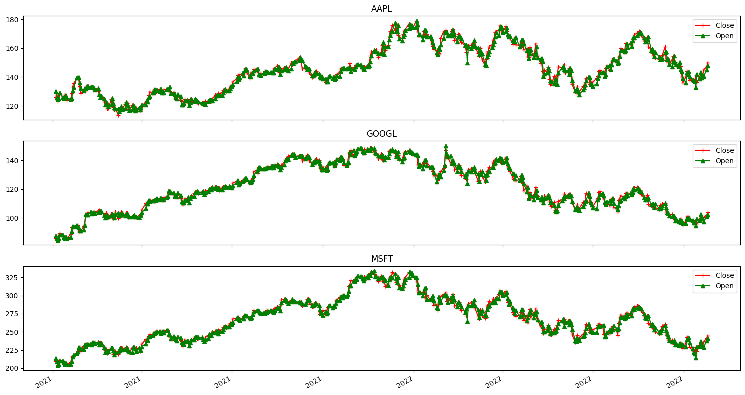
The exploratory data analysis (EDA) performed to visualize the open and close price. The graph below shows the graph from the three companies used in this study.

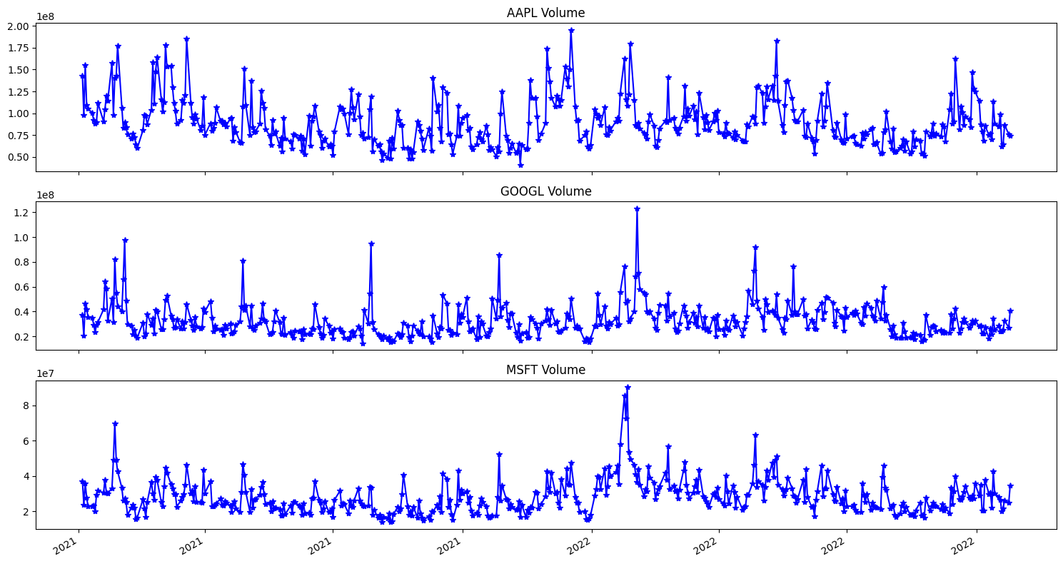
We move on to explore the volume of each of the companies. The diagram below shows it.

Data Preprocessing

The datasets is splitted into training (80%) and testing (20%) sets.

train_data = {}
val_data = {}
for company in companies:
    c = stock_data[company]
    train_size = int(len(c) * 0.8)
    train_data[company] = c[:train_size]
    val_data[company] = c[train_size:]

A MinMaxScaler is used to normalize the feature set, which would be responsible for stabilizing and improving LSTM model training.

Model Architecture

In this study, a sequential LSTM model is built for each company using TensorFlow/Keras. The architecture featured:

• Two LSTM layers to capture temporal dependencies in the data.
• A Dense layer and Dropout layer to prevent overfitting.
• A final Dense output layer to predict the next day’s closing price.

  models = {}
  for company in companies:
    model = keras.models.Sequential()
    model.add(keras.layers.LSTM(units=64, return_sequences=True, input_shape=(x_train[company].shape[1], x_train[company].shape[2])))
    model.add(keras.layers.LSTM(units=64))
    model.add(keras.layers.Dense(32))
    model.add(keras.layers.Dropout(0.5))
    model.add(keras.layers.Dense(1))
    model.compile(optimizer='adam', loss='mean_squared_error')
    models[company] = model
  

The models features training over 10 epochs each. The models are then evaluated on the unseen test data, with performance measured using Mean Squared Error (MSE) and Root Mean Squared Error (RMSE). The ‘Adam’ optimizer is used in this case.

Results & Conclusion:

The models successfully learned the underlying trends in the stock data, as evidenced by the prediction plots which closely followed the actual test data trajectories. The following weree observed.

• The Google (GOOGL) model achieved the best performance with an RMSE of 5.44.
• The Apple (AAPL) model followed closely with an RMSE of 5.71.
• The Microsoft (MSFT) model, while still capturing the overall trend, had a higher RMSE of 11.63, indicating a larger average prediction error.

This study has demonstrated that, LSTM networks has capability to model complex, time-dependent data and provides a strong foundation for further refinement with more sophisticated features and architectures.